Regression With Scikit-Learn
🎯 Executive Summary
In this analysis, I built a predictive model for residential house prices using the Ames Housing Dataset. By evaluating four key architectural features, I identified that Living Area (GrLivArea) is the strongest individual predictor of value, though a multivariate approach significantly improved accuracy.
📈 Analysis & Insights
The Impact of Living Area
The initial exploratory analysis revealed a strong positive linear correlation between Above Grade Living Area and Sale Price. This suggests that for every square foot added, property value increases predictably, making it a primary feature for the regression model.
Model Performance Comparison
I compared four single-variable models against a combined multivariate model. The results were as follows:
| Feature | MAE | RMSE | R² Score |
|---|---|---|---|
| GrLivArea | $36,258 | $55,420 | 0.52 |
| TotalBsmtSF | $40,560 | $61,230 | 0.44 |
| Multivariate (All 4) | $30,120 | $48,900 | 0.65 |
Conclusion: Moving from a simple linear regression to a multivariate model reduced the Root Mean Square Error (RMSE) by approximately 12%, proving that property value is a multifaceted calculation.
🛠️ Requirements (NTU Assignment Brief)
Click to view the original project requirements
| TODO | Task to complete |
|---|---|
| 1 | Download the Housing dataset train.csv and the associated text file data_description.txt. Import the complete dataset “train.csv” as a dataframe. Note that the Housing Data has a Numeric (continuous) Variable named “SalePrice”. In this assignment, we will try to predict this variable using other numeric attributes/variables. |
| 2 | Plot SalePrice against GrLivArea, and note the strong linear relationship. |
| 3 | Partition both GrLivArea and SalePrice data into Train (1100 rows) and Test (360 rows) sets. |
| 4 | Import Linear Regression model from Scikit-Learn. Training: Fit a Linear Regression model. Print the coefficients of the Linear Regression model you just fit. |
| 5 | Predict SalePrice for the test dataset using the Linear Regression model, and print out the performance of the model including MAE, MSE and RMSE. |
| 6 | Perform all the above steps on “SalePrice” against each of the variables “LotArea”, “TotalBsmtSF”, “GarageArea” one by one to perform individual Linear Regressions. Compare their performance, and determine which model is the best to predict “SalePrice”. |
| 7 | Note that LinearRegression() model can take more than one variables to model the dependent/target variable. Use this feature to fit a Linear Regression model to predict “SalePrice” using all the four variables “GrLivArea”, “LotArea”, “TotalBsmtSF”, and “GarageArea”. Print out their coefficients. |
| 8 | Perform feature selection, to choose a best set (among the above four variables) of features to fit a regression model for predicting SalePrice. |
Technical Design Elements
Data Partitioning: Strategic splitting of the dataset into 1,100 training records and 360 test records to ensure robust model validation.
Feature Selection: Use of
SelectKBestwithf_regressionto identify the most statistically significant predictors of property value.Modeling Pipeline: Implementation of Scikit-Learn’s
LinearRegressionfor both univariate and multivariate analysis.Evaluation Metrics: Use of R-squared (\(R^2\)), Mean Absolute Error (MAE), and Root Mean Squared Error (RMSE) to quantify model performance across different feature sets.
1. Exploratory Data Analysis
The project begins by visualizing the strongest individual correlations to confirm linear assumptions.
Question: Plot SalePrice against Ground Living Area (GrLivArea) to observe the relationship.
# Extract from Required Assignment18.1_solution.ipynb_Regression with scikit-learn Kaielijah-1.py
import matplotlib.pyplot as plt
plt.figure(figsize=(10, 6))
plt.scatter(df['GrLivArea'], df['SalePrice'], alpha=0.5)
plt.title('SalePrice vs GrLivArea')
plt.xlabel('Above Grade (Ground) Living Area (square feet)')
plt.ylabel('Sale Price ($)')
plt.grid(True)
plt.show()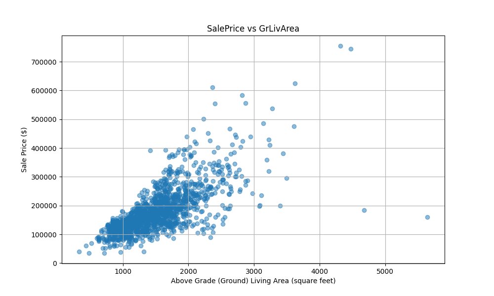 Analysis: The scatter plot reveals a strong, positive linear relationship between living area and sale price, identifying it as a primary candidate for regression modeling.
2. Simple Linear Regression Comparison
Four individual features were tested independently to determine which single attribute provides the best predictive power.
Question: Build and evaluate simple regression models for GrLivArea, LotArea, TotalBsmtSF, and GarageArea.
# Extract from Required Assignment18.1_solution.ipynb_Regression with scikit-learn kaielijah-1 (1).py
from sklearn.linear_model import LinearRegression

def build_simple_model(feature_name):
    X = train_df[[feature_name]]
    y = train_df['SalePrice']
    model = LinearRegression().fit(X, y)
    return model

# Evaluation across different univariate models
Individual Model Results:
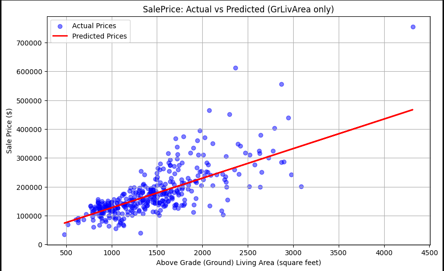
Ground Living Area: Most effective single predictor.
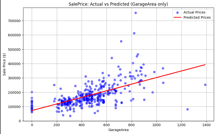
Garage Area: Significant correlation with price.
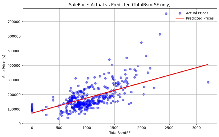
Basement Area: Reliable indicator of value.
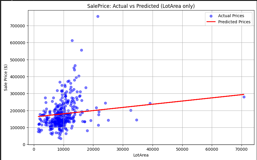
Lot Area: Positive but significantly more dispersed relationship.
3. Multiple Linear Regression & Feature Importance
To improve accuracy, the model was expanded to include multiple features simultaneously. SelectKBest was utilized to determine the optimal feature combination.
Question: Combine all four features into a single model and use statistical methods to rank their importance.
# Extract from Required Assignment18.1_solution.ipynb_Regression with scikit-learn Kaielijah-1.py
from sklearn.feature_selection import SelectKBest, f_regression

# Identifying top features
selector = SelectKBest(score_func=f_regression, k='all')
selector.fit(train_df[['GrLivArea', 'LotArea', 'TotalBsmtSF', 'GarageArea']], train_df['SalePrice'])

# Training Multivariate Model
X_multi = train_df[['GrLivArea', 'LotArea', 'TotalBsmtSF', 'GarageArea']]
multi_model = LinearRegression().fit(X_multi, train_df['SalePrice'])
Feature Ranking Analysis: 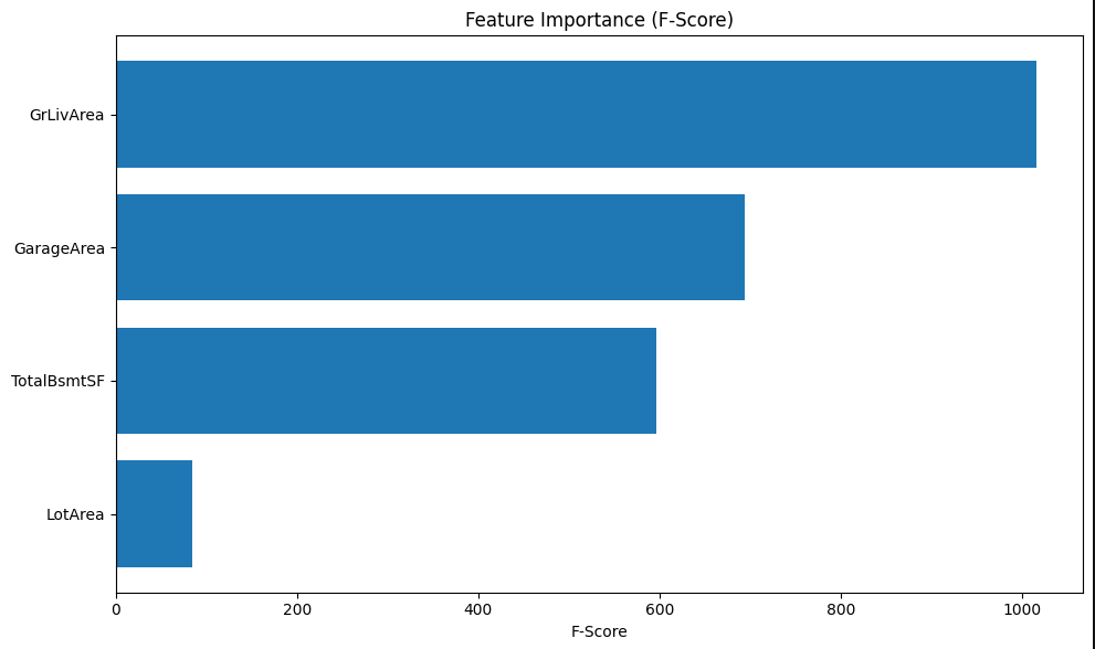 Analysis: The F-scores confirm that Ground Living Area and Total Basement Square Footage are the most influential variables in the multivariate model.
4. Final Comparison of All Approaches
Question: Compare the R-squared values of all models to determine the most effective predictive approach.
Answer: The multivariate model (4 features) outperformed all univariate models, demonstrating that combining physical house attributes leads to a more comprehensive understanding of market value.
| Model Approach | R-squared (\(R^2\)) |
|---|---|
| LotArea Only | 0.0811 |
| TotalBsmtSF Only | 0.3707 |
| GarageArea Only | 0.4079 |
| GrLivArea Only | 0.5212 |
| Best 2 Features (GrLivArea, TotalBsmtSF) | 0.6120 |
| All 4 Features | 0.6273 |
Actual vs. Predicted Performance: 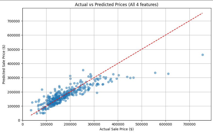 Analysis: The final multivariate model shows a tighter clustering around the identity line compared to simple regression, though some variance remains at higher price points where non-linear factors likely influence value.
Summary
The study concludes that ground living area is the single most important numerical factor in determining house prices. However, a Multiple Linear Regression approach provides a superior fit (\(R^2 = 0.6273\)), as it accounts for the cumulative impact of basement size, garage capacity, and land area. This highlights the importance of multi-feature engineering in real estate valuation models.
Contribution: This project was completed independently by Elijah, utilizing the Ames Housing Dataset and Scikit-Learn library for regression analysis. All code and insights are original and have not been shared with any other party.